About this part
This part starts from a finished model, as described in Part 1 (Modeling). It covers:
- how to set up studies, which are the analyses you want to run;
- the five analysis types and their settings;
- load cases and load combinations in the results;
- the mesh and the solvers, including high-order solid elements;
- how to run a study;
- how to read the results in the 3D view, the Results panel, tables and charts;
- how to export results.
Part 3 (Design) continues from a solved static study. In this part, menu commands are written as Menu › Group › Command, and keys are shown like F5.
Studies
A study is one analysis of the model: its type and its settings. A project can hold several studies, for example a linear static study for design and a modal study for the natural frequencies. Studies are listed under stage 4 Analysis in the Explorer. Each one shows its type as a badge, and the stage shows whether it has been run.
Analysis types
FEA Studio has five analysis types. All of them run on the built-in Project Chrono solver; linear static and modal studies of solid models can also run on MFEM with high-order elements (see "Solvers").
| Analysis menu | Study type | What it does |
|---|---|---|
| Linear static | Static | Linear elastic analysis with small displacements: one solution per load case, or one combination |
| Modal | Modal | Natural frequencies, periods and mode shapes |
| Linear dynamic | Dynamic | Linear transient response to loads applied at t = 0, integrated in time (HHT) |
| Nonlinear static | Nonlinear | Large-displacement static analysis in load increments, with Newton–Raphson iterations in each |
| Response spectrum | Response spectrum | Modal combination (SRSS or CQC) of a code design spectrum |
Note. FEA Studio has no separate buckling or P-Δ study type. Use a Nonlinear static study when large displacements matter; the steel design settings offer member and storey sway amplification (Part 3).
Adding a study
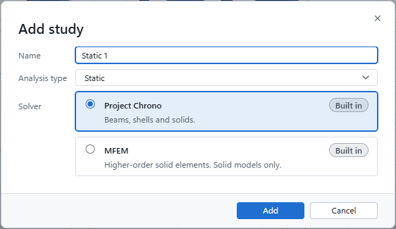
- In the Explorer, right-click the Analysis stage and choose Add study.
- In Add study, type a Name. It follows the type until you edit it, for example "Static 2".
- Choose the Analysis type.
- For Static and Modal, choose the Solver: Project Chrono (beams, shells and solids) or MFEM (higher-order solid elements, for solid models only).
- Click Add. The new study is selected so you can set its options in Properties.
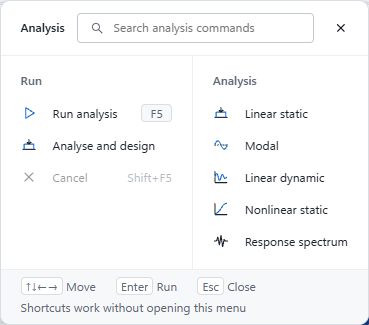
You can also skip this dialog. Analysis › Analysis › Linear static (or Modal, Linear dynamic, Nonlinear static, Response spectrum) runs the first study of that type, and creates one with default settings if none exists.
Right-click a study for Run study, Rename (F2), Delete and Properties. Drag studies to change their order.
Study settings
Select a study to see its settings in Properties. The Study group holds the name and the analysis type; the type can be changed later. The other settings depend on the type:
| Setting | Study types | Meaning (default) |
|---|---|---|
| Solve | Static | Each load case: one solution per load case, plus the code load combinations and their envelopes; the design modules use these. One combination: a single solution of the combination below. |
| Load combination | Static (one combination), Dynamic, Nonlinear, Response spectrum | For example 1.35 Dead + 1.5 Live. Empty means every load once. |
| Mass from load cases | Modal, Response spectrum, Dynamic | For example 1 Dead + 0.25 Live. Self-weight is always counted as mass. |
| Number of modes | Modal | Lowest modes to find (6) |
| Duration · Time step | Dynamic | 1 s · duration / 200. Use a step of about 1/20 of the shortest period of interest. |
| Rayleigh β | Dynamic | Stiffness-proportional damping in seconds; the damping ratio is about β·ω/2 (0 = undamped) |
| Member force history | Dynamic | Keep member forces at every output frame (larger result files) |
| Plastic hinges | Dynamic | Plastic hinges at the ends of tubular members (plastic moment with the N–M interaction), for blast and impact; with a limit displacement |
| Load increments | Nonlinear | Load steps, each solved with Newton–Raphson (10) |
| Solver · Element order | Static, Modal | Project Chrono or MFEM; with MFEM, the element order: 1 = linear, 2 = quadratic (default), 3–4 = cubic, quartic |
Tip. For design, use a Static study with Solve: Each load case. Each load case is then solved once, and the code combinations and envelopes are built from those solutions without solving again. That is what the design modules need.
Analysis settings
Expand the Analysis stage in the Explorer and double-click Settings (or choose Analysis settings… from it). The Analysis settings dialog lists every study with its Solver. A study whose type only one solver can run says so. Changing a solver does not remove results already run. The badge beside Settings shows the solvers in use, for example Chrono.
Response spectrum studies
A response spectrum study is made from the code spectrum:
- Choose Assign › Generate › Response spectrum.
- Pick the code, then enter the seismic inputs (as for Earthquake loads; see Part 1).
- In Response spectrum study, set the options below, then click Create.
| Field | Default |
|---|---|
| Direction factors X Y Z | 1 0.3 0 |
| Combination of directions | 100-30 or SRSS |
| Modes | 30 |
| Damping ratio (CQC) | 0.05 |
| Scale up to NN % of the static base shear | On (ASCE 7 and KDS) |
| Use each direction as an earthquake load case in design | Gives the load cases Seismic RSA X and Seismic RSA Y |
The study is named Response spectrum. Running the command again updates it. Analysis › Analysis › Response spectrum runs the first response spectrum study, or makes one from the code spectrum first.
Load cases and combinations
Every load of the model belongs to a load case, and every case has a category such as Dead, Live, Wind or Earthquake (Part 1). The analysis uses them in two ways:
- A Static study solved Each load case gives one result per load case, and builds the load combinations of the design code from those results.
- A study with a Load combination (for example
1.2 Dead + 1.6 Live) solves that one combination. A study with no combination applies every load once.
Define › Load cases › Load combinations chooses which code combinations are used and lets you add your own (see Part 3). The dialog stays available after solving: when you change it, the combination results are rebuilt at once, without solving again.
In the results, the case selector is grouped as follows:
- Load cases
- Strength combinations
- Service combinations
- Envelopes
Your own combinations are marked (yours). An envelope shows, for each value, the largest or smallest result over the strength or service combinations. The deformed shape of an envelope is therefore not one real load state.
The mesh
The solvers work on the mesh, not on the geometry you draw. You do not have to build it yourself: when you run a study, the mesh is generated first if there is none, or if the model changed since it was built (Part 1 describes the mesh settings).
- Beams, trusses and cables become line elements; surfaces with a thickness become shell elements; solids become tetrahedra or hexahedra.
- Mesh › Generate › Settings sets the element size, quadrilateral or triangular shells, and hexahedral or tetrahedral solids.
- Mesh › Inspect › Check quality opens the Mesh quality panel. Check the worst elements of a solid model before you trust its stresses.
- The status bar shows Mesh: none, out of date or up to date.
Solvers
| Solver | Kind | Used for |
|---|---|---|
| Project Chrono | Built in | Beams, trusses, cables, shells and solids: Linear static, Modal, Linear dynamic, Nonlinear static and Response spectrum |
| MFEM | Built in | Higher-order solid elements (order 1–4) for Linear static and Modal. Solid models only: tetrahedra and hexahedra, no beams or shells. |
| CBFEM | Built in | Steel connections: a shell model of the plates, bolts and welds of each connection (Part 3) |
High-order solids (MFEM)
Linear elements are stiff in bending and under-estimate stress peaks unless the mesh is very fine. MFEM solves the same tetrahedral or hexahedral mesh with higher-order elements, which gives far more accurate stresses in bending and at stress concentrations.
- Mesh the solids (Part 1). Every element must be a tetrahedron or a hexahedron.
- Add a Static or Modal study and choose MFEM as the Solver, or change the solver of an existing study in its Properties or in Analysis settings.
- Set the Element order in the study's Properties: 2 (quadratic) is the default. Each step up multiplies the number of equations by about 2–3 for tetrahedra and 3–4 for hexahedra.
- Run the study as usual.
If the model also has beams, trusses or shells, the Solver field says that MFEM handles solid models only; use Project Chrono for those models.
Note. In the browser version, analyses are sent to the local solver server. Without it, a run stops with the message that it needs the desktop app or the solver server.
Running an analysis
Ways to run
| Command | Runs |
|---|---|
F5 · Analysis › Run › Run analysis | The study selected in the Explorer, or else the first static study |
| Run linear static ▾ on the toolbar | The first linear static study; the drop-down picks another type |
| Analysis › Analysis › Linear static / Modal / Linear dynamic / Nonlinear static / Response spectrum | The first study of that type, made with defaults if none exists |
| Right-click a study › Run study | That study |
| Run analysis in the empty Results panel | As F5 |
| Analysis › Run › Analyse and design | Makes the design objects, solves the load cases and designs everything in one go (meant for models imported from IFC; see Part 3) |
What happens when you run
- The mesh is checked. If there is no mesh, or the model changed since it was built, the mesh is generated first. The Output panel says so.
- The model is validated. Problems such as missing sections or no supports are listed in the Output panel. If there is an error, a message names the study and the problem, and nothing runs.
- A progress card appears. It shows the percentage, the current stage, the elapsed time and an estimate of the time left. Click Cancel, or press
EscorShift+F5, to stop the run. You can hide the card with ×; the status bar keeps showing the progress, and clicking it brings the card back. - When the run finishes:
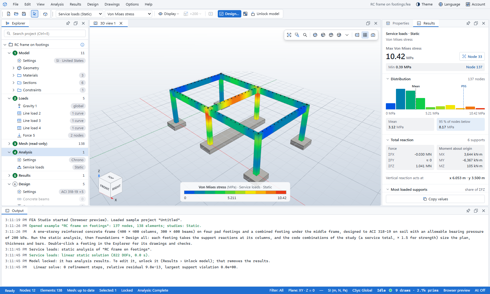
- the Output panel lists the solver's messages;
- the Results panel opens and shows the new result set;
- the model is locked.
If the run fails or you cancel it, the message is shown in the Output panel and the status bar reads Failed or Cancelled. Only one analysis can run at a time.
The status bar
Analysis: in the status bar shows Idle, Running…, Complete, Cancelled or Failed. While a study runs, it shows the study name, the percentage and the stage. Click it to see the progress card, or the Output panel when nothing is running.
Locked models
A model with results is locked, so the results always belong to the geometry you see. The status bar says Locked, and editing commands are greyed out.
- Unlock model (Results › Lock, or the Results toolbar) asks for confirmation, then removes all result sets and makes the model editable. Solve again after editing.
- Design objects such as beam lines and footings stay, and their settings stay editable while the model is locked.
Reading the results
The Results toolbar
After an analysis, the Results toolbar replaces the modelling toolbars. From left to right it has:
| Control | What it does |
|---|---|
| Result set | Chooses which solved study and case to show, or (none: show the model) |
| Quantity | The contour to plot (see the table below) |
| Case / mode / time | The load case or combination, the mode, or a time slider, depending on the study |
| Display ▾ | Deformed shape, overlay of the undeformed model, reactions, smooth and banded contours |
| Deformation scale ▾ | ×N; Auto draws the largest displacement at about 8 % of the model size |
| Animate | Animates mode shapes, dynamic results or the deformation |
| Design…, D/C ratios | Design (see Part 3) |
| Unlock model | Makes the model editable again; this removes the results |
Quantities
| Group | Quantities |
|---|---|
| Displacement | Displacement |u|, Displacement X / Y / Z, Rotation |θ| |
| Stress | Von Mises stress, Max principal stress, Min principal stress |
| Strain | Equivalent strain, Plastic strain |
| Member forces | Axial force N, Bending moment |M|, Shear force |V|, Torsion T |
| Motion | Velocity |v|, Absolute acceleration |a| (dynamic studies) |
| Temperature | Temperature change |
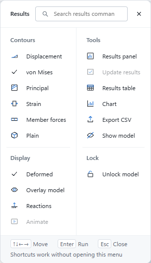
Only quantities that the result set contains are listed. The Results › Contours menu has shortcuts: Displacement, von Mises, Principal, Strain, Member forces and Plain (the shape without contours).
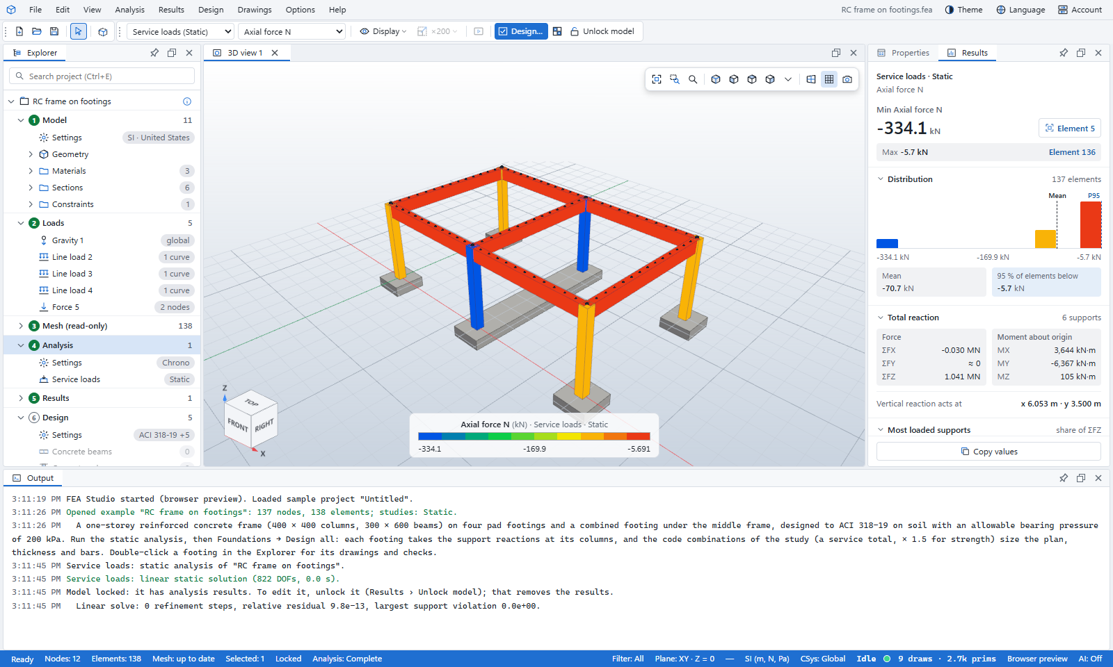
Note. Member forces are shown as colours along the members, not as moment or shear diagrams. For numbers at member ends, use Results table, Export CSV or the Analysis report.
Deformed shape
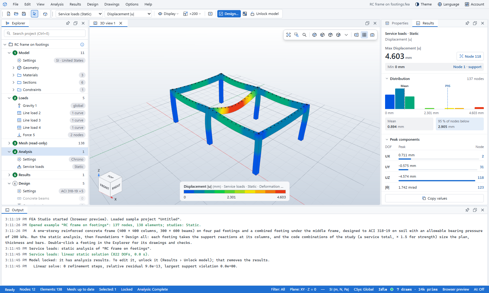
FEA Studio draws the model deformed only when the contour is a displacement quantity, or when there is no contour. Stresses, strains and member forces are drawn on the undeformed model, so the colours sit where the material actually is. This rule is the reason the Deformation scale control is greyed out for stress plots.
- Display ▾ › Deformed shape turns the deformation on or off.
- Overlay undeformed model shows the original shape as well.
- Deformation scale ▾ offers Auto, ×1 (true scale), ×10, ×100 up to ×5000, or a custom factor.
Animation
Animate (Results › Display) plays:
- mode shapes swinging back and forth;
- static shapes growing from zero to full;
- linear dynamic and nonlinear static results frame by frame, in a loop.
Animation stops when you switch to a quantity that is not a displacement. Load arrows are hidden while an animation plays.
The legend
The colour legend sits at the bottom centre of the 3D view. It shows:
- the quantity and its unit;
- the study, the case or frame, and the deformation scale;
- the minimum and maximum values.
Hover over the bar to read a value. With Banded on, it has 10 bands; otherwise the colours are smooth.
Colour scales
Options › Display › Colour scale chooses the colours of every contour. Your choice is kept for next time.
- Standard: FEA Studio (blue–green–yellow–red, the default), Abaqus (12 bands), Rainbow, Jet, Turbo, Cool to warm, Black body, Grayscale.
- Pastel: pastel versions of the standard scale, rainbow and cool to warm.
- Colour-blind safe: Viridis, Plasma, Inferno, Cividis, Blue–white–red, Blue–orange.
- Reversed flips any scale.
Options › Display › Colour map… gives finer control:
- the number of Bands (0 = smooth);
- Logarithmic scaling;
- the Range: Frame shown, All frames, Visible (leaves out hidden and clipped parts), or Custom with your own minimum and maximum.
The Results panel
The Results panel (right, beside Properties) summarises the result shown:
- The headline: the study and the quantity, the largest value with its unit, and the node or element where it occurs. Click the node or element button to select and zoom to it. The opposite extreme is shown below it.
- Distribution: a histogram of the values over the nodes or elements, with the mean and the value 95 % of them stay below.
- Peak components (displacements): the largest UX, UY, UZ and rotation, each with its node.
- Total reaction: the sums ΣFX, ΣFY, ΣFZ at the supports and their moments about the origin, where the vertical reaction acts, and the most loaded supports. The sums are a quick equilibrium check against the applied loads.
- Copy values copies the panel's numbers to the clipboard.
Select a node or element in the 3D view to see its own values in the panel. Sections can be folded away; values too small to matter show as ≈ 0.
Reactions
Results › Display › Reactions draws reaction arrows at the supports. The totals are in the Results panel, and the reactions at every support node are in the Results table, the Analysis report and the CSV export.
Results table
Results › Tools › Results table lists every result of the frame shown, at the nodes or elements. You can sort and filter the columns; the table follows the selection in the 3D view, and it can be saved as CSV.
Charts
Results › Tools › Chart opens a chart in the main area, as a tab beside the 3D view.
| Chart | Shows |
|---|---|
| Frequencies | Natural frequencies of a modal study as bars |
| History / Per mode | A value of the selected node (or the node with the largest value) over time, load increments or modes |
| Along selection | Values along a path. Select two or more nodes in order with Ctrl+click. |
The chart can be saved with CSV or SVG, or sent to Print, PDF or Word.
Several result sets
Each solved study keeps its own result set under stage 5 Results in the Explorer. Activate a row to show it, or use the Result set selector. Right-click › Remove deletes a result set; removing the last one unlocks the model. Results › Tools › Show model hides the results and shows the plain model, which stays locked.
Exporting results
| Command | Output |
|---|---|
| Results › Tools › Export CSV | The frame shown, as a CSV file: node coordinates and displacements; element stresses and strains; beam end forces N, Vy, Vz, T, My, Mz at both ends; support reactions |
| Results › Tools › Results table › CSV | The table as shown, with your sorting and filters |
| File › Export › VTK (.vtk) | The mesh with the shown results, for ParaView and similar tools |
| File › Export › Nodes (CSV), Elements (CSV) | The mesh tables |
| File › Export › IFC with results (.ifc) | The building model with the analysis results attached (Part 1) |
| File › Export › Viewport image (PNG) | A picture of the 3D view as shown |
| Chart › CSV, SVG, Print, PDF, Word | The chart and its data |
| File › Reports › Analysis report | The full analysis report (see Part 5) |
Troubleshooting
| Message or symptom | What to do |
|---|---|
| "(study name) can't run" with an error in Output | Read the Output panel. Usually a member has no section, a shell has no thickness, or the model has no supports. |
| Very large displacements, or a "singular" warning | The model is a mechanism: check supports, released ends and unconnected nodes. Mesh › Display › Show mesh and Mesh nodes help to find gaps. |
| "An analysis is already running" | Wait for it, or press Esc to cancel it. |
| Results look stale | The Results panel warns when the mesh differs from the one that was solved. Unlock, then run again. |
| Can't edit the model | It is locked by its results. Use Unlock model. |
| MFEM is not offered, or says solid models only | The model has beams, trusses or shells, or the study is not Static or Modal. Use Project Chrono. |
| Browser: "needs the desktop app, or the solver server" | Start the solver server, or use the desktop app. |
| Netgen not available | Netgen needs the desktop app or the solver server. |